
IPM Basics
An Intra-population Model (IPM) describes the behavior of an infectious disease within a population. IPMs encode compartmental models, which is one common modeling method in epidemiology. In compartmental models, populations are simulated as groups of anonymous individuals who are characterized primarily by which disease state they are in at any given point in time.
To define a compartmental model, you define the different states in which an individual can exist (compartments), as well as expressions for the instantaneous rates of change between each state (events), which can be parameterized by external data requirements (parameters).
Compartmental modeling example
This is a classic “SIRS” model, represented as a directed graph:
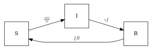
This model structure is commonly used for simplistic modeling of a pathogen with human-to-human transmission. Individuals may start out susceptible to acquiring the pathogen (\(S\)). Then there is a period of infection (\(I\)) during which individuals can spread the pathogen to others. And finally there is a period of immunity (\(R\)) during which individuals are assumed to have no chance of becoming reinfected. This immunity may go away over time, or wane, due to the immune system “forgetting” the pathogen or because the pathogen mutates to escape prior immunity, which cycles the individual back to susceptible. (The last “S” in the name SIRS indicates the presence of this cycle.)
TipInfection versus infectiousness
In this model, “infected” also implies “infectious”, but this is not necessarily the case in more complex models! Many real diseases have a period of incubation where individuals have been infected (exposed) but are not yet capable of spreading that infection to others. Be careful to make that distinction when it is needed.
Along each directed edge of this graph is the expression for the rate of transition for individuals from one state to another. These expressions are often written in terms of the number of individuals in the compartments (\(S\), \(I\), and \(R\)) as well as scalar parameters to modulate the rates of change (\(\beta\), \(\gamma\), and \(\xi\); that is, beta, gamma, and xi). If we consider the inflows (positive) and outflows (negative) from each compartment, we can convert this into a system of ordinary differential equations with respect to time:
\[ \begin{aligned} \frac{dS}{dt} &= - \frac{\beta S I}{N} + \xi R \\[10pt] \frac{dI}{dt} &= + \frac{\beta S I}{N} - \gamma I \\[10pt] \frac{dR}{dt} &= + \gamma I - \xi R \end{aligned} \]
(Where \(N\) is a notational convenience for the total number of individuals, equal to \(S + I + R\).)
Given these differential equations and if we know the initial values of \(S\), \(I\), and \(R\), we can obtain the trajectories of \(S(t)\), \(I(t)\), and \(R(t)\) by computing the integrals. Rather than attempt to solve integrals analytically, which could become overwhelming for more complex models, epymorph approximates integrals using Tau Leaping. This allows us to efficiently simulate a stochastic system using integer values. The result might look a little like this (for a single location RUME):
In the process of an epymorph simulation, applying the IPM is a separate step from applying movement. Indeed, the fact that tau leaping gives us natural “seams” in which to interpose our movement dynamics was another key reason for choosing this method. We will cover movement in more detail in a later section. For now, understand that during each time step, the IPM is applied to the population that is present in every location independently. Hence “intra” in the name Intra-population Model. epymorph assumes that individuals at the same location have an equal probability of interacting with one another: they are “well mixed”. They also have zero probability of interacting with individuals at other locations. It is the movement model which is responsible for “remixing” populations such that a pathogen might spread from location to location.
TipModel stratification
This chapter focuses on IPMs with a single stratum. With a single stratum IPM, we are implying that all individuals are affected by the pathogen in the same way. It is common, though, for real pathogens to affect individuals differently based on their characteristics. For instance, influenza is noted to result in hospitalization more often for older adults than for younger adults. In this case we may wish to “stratify” the population: divide the population by critical characteristics such that we can apply different parameter values to each (like \(\beta\)), or even entirely different compartmental model structures. These multistrata models will be covered in a later chapter.
Defining IPMs
epymorph provides a library of built-in IPMs for some commonly-used models, but you will very likely want to define your own.
Here is the source code for the SIRS model used above, with added in-line explanation, describing the process of defining an IPM.
# Define a class extending the `CompartmentModel` base class
class SIRS(CompartmentModel):
    """A basic SIRS model."""

    # First define compartments as a class attribute,
    # and provide a list of `CompartmentDef` instances
    # using the utility function `compartment()`.
    # Specify (at least) the symbol to use for each compartment,
    # which will double as its name.
    compartments = [
        compartment("S"),
        compartment("I"),
        compartment("R"),
    ]

    # Next define the data requirements, or parameters,
    # that our IPM's transition expressions will use.
    # The beta, gamma, and xi parameters in this model can all
    # vary over time and between location, so they are given the
    # shape "TxN". Individual values are floating point numbers,
    # give them type "float". And each has a comment which is used
    # to describe the parameter to users of the IPM.
    requirements = [
        AttributeDef(
            "beta",
            type=float,
            shape=Shapes.TxN,
            comment="infectivity",
        ),
        AttributeDef(
            "gamma",
            type=float,
            shape=Shapes.TxN,
            comment="progression from infected to recovered",
        ),
        AttributeDef(
            "xi",
            type=float,
            shape=Shapes.TxN,
            comment="progression from recovered to susceptible",
        ),
    ]

    # Last, specify the transitions, or edges, that connect
    # the model's compartments and allow individuals to progress from
    # one state to another.

    # To do this, define the `edges()` method.
    # It will be called by epymorph internally when the IPM
    # is instantiated.
    def edges(self, symbols):
        # The method will be passed an argument called `symbols`,
        # which contains objects (sympy symbols) representing
        # the compartments and parameters declared above.
        [S, I, R] = symbols.all_compartments
        [β, γ, ξ] = symbols.all_requirements

        # If needed, create useful sub-expressions to make the
        # code more readable, leveraging the sympy library.
        # sympy lets you use standard standard mathematical syntax
        # to combine symbols into expressions.

        # Here is an expression for computing `N`
        # (the total population in all compartments)
        # formulated so as to avoid dividing by zero
        # in case a location's population ever goes to zero.
        # sympy's `Max()` function helps us here.
        N = Max(1, S + I + R)

        # Finally, return a list of `EdgeDef` instances, one for each
        # directed edge in the graph, using the `edge()` utility function.
        # Specify the "from" and "to" compartment for each edge
        # as well as the rate expression.
        return [
            edge(S, I, rate=β * S * I / N),
            edge(I, R, rate=γ * I),
            edge(R, S, rate=ξ * R),
        ]
You will find API reference for all of these classes and functions in the compartment_model module.
Once you understand how this IPM is constructed, you can define your own by copying this class into your own script and modifying it to fit your needs. Copy-and-modify is a great way to get started.
Say, for example, that you wanted to model the effects of vaccination. Starting from the SIRS model, you would add a Vaccinated compartment. If you want people to get vaccinated at a certain rate during the simulation, or for the effects of the vaccine to wane over time, add edges to account for those inflows and outflows. And to give the model flexibility in expressing these dynamics, add model parameters for these edges. This is just one idea for a basic IPM variant; IPMs can be arbitrarily complex!
When it’s time to set up and run a simulation, you would use a custom IPM in a RUME in exactly the same way as you would use a built-in IPM.
IPM features in detail
The IPM listed above is a good starting example, but it doesn’t use every feature available in epymorph. Here we’ll take a detailed look at all of the options for IPM construction.
Validation
CompartmentModel subclasses are subjected to validation upon definition. You may see an IPMValidationError raised at class definition time if there are structural problems with your IPM, and the message should guide you towards the problem. For example, an IPM with duplicate compartment names is considered invalid, and you should fix that by defining unique names for each.
Compartments
IPMs must define at least one compartment. Compartment names must start with a letter (lowercase or uppercase) and can contain only letters, numbers, dashes, and underscores. Compartment names must be unique, and their definition order is used as their canonical ordering, e.g., by the initializer, in the simulation output, and when drawing plots.
Compartments are defined by instances of the CompartmentDef class, but constructing these directly can be tedious, so the compartment() function is provided as a convenient alternative constructor.
You may use a subscripted name, such as I_symptomatic or I_asymptomatic, to distinguish related states. The first underscore in the name separates the “base” part of the name from the subscript part. This type of naming scheme is conventional in epidemiology, but additionally, subscripts are given special treatment in some epymorph features. For example, when making IPM quantity selections for plotting: rume.ipm.select.compartments("I_*") uses an asterisk as a wild card to select all “I” compartments, regardless of subscript.
You can define tags on compartments. Tags are intended to support specialized logic per compartment. As of epymorph v1.2.0, the only tag which has any real effect on the simulation is "immobile". A compartment tagged immobile will be ignored during the movement processing phase, such that individuals in this compartment will not be subject to movement. This is particularly useful for modeling hospitalization, for instance. Support for additional tags may be added in the future.
Compartments can include a human-readable description to help users understand the IPM.
The following example showcases all of the above features:
compartments = [
    compartment("S", description="Susceptible"),
    compartment("I_asymptomatic", description="Infectious (Asymptomatic)"),
    compartment("I_symptomatic", description="Infectious (Symptomatic)"),
    compartment("R", description="Recovered"),
    compartment("H", description="Hospitalized", tags=["immobile"]),
]
Remember that compartments are one of the results quantities that you can select for plotting and data processing, so you may wish to refer back to that section as well.
Parameters
An IPM may declare zero or more data requirements that will need to be supplied as RUME parameters for the IPM to function. These parameters are useful tools for influencing the transition rates in response to external data, and make your IPM reusable in ways it would not otherwise be.
Requirements are defined as AttributeDef instances. Each specifies a parameter name, data type, maximal shape, optional default value, and optional descriptive comment. Data shapes allowed for use in IPM requirements are somewhat restricted; requirements must use one of the following shapes:
Scalar: a scalar value,T: (time) an array of values per day,N: (node) an array of values per location, orTxN: (time-by-node) an matrix of values per day and location.
Similarly, all data types must be either int or float, because these values will be used directly in mathematical expressions.
Requirements of an IPM will use the "ipm" module for the sake of RUME parameter namespacing. For example, providing a value with name "*::ipm::beta" targets IPM requirements named “beta” across all strata. (See RUME Parameters for more information.)
Designing model parameters is somethign of an art, and a lot of flexibility is given to you as the author. The example used fairly generic, scalar parameters for modulating transition rates, but parameters can be used to integrate concrete factors like temperature and humidity. You can decide to include those factors in your IPM rate expressions directly, or you might prefer to keep the parameters generic and compute the values provided to the RUME in such a way as to integrate those factors. It depends on your use-case and stylistic preferences. Being specific is less reusable but more explicit, while being general is more reusable and less explicit.
Transitions
To define the transitions in your IPM, your class implements the edges(self, symbols) method, whose method body constructs and returns the transition definitions as TransitionDef instances.
Acquiring symbols
The symbols argument provides SymPy symbols for the declared compartments and requirements. You can retrieve them in declaration order with symbols.all_compartments and symbols.all_requirements. Or if you prefer, you can retrieve them by name using the symbols.compartments() and symbols.requirements() methods, for which you specify the names in the order you expect to use them. This is more explicit and for that reason, somewhat safer.
For the SIRS model shown above, all of the following are equivalent:
[S,I,R] = symbols.all_compartments

[S,I,R] = symbols.compartments("S", "I", "R")

[R,S,I] = symbols.compartments("R", "S", "I")

# or, if you don't want to use Python's destructuring assignment feature:
csymbols = symbols.all_compartments
S = csymbols[0]
I = csymbols[1]
R = csymbols[2]
Transition rate expressions
The transition rate for an edge is the expected average number of individuals that should make that transition per day. (For tau steps smaller than one day, the effective rate is the daily rate divided by the length of the tau step.) It it important to keep in mind that IPMs involve stochastic computation: if your rate evaluates to “1000 events per day”, you may see somewhat more or less events on a particular day. Tau leaping uses a Poisson random variable for this, and, in this case, 1000 is the mean of the distribution.
TipWhat happens if the rate is larger than the number of individuals in the source compartment?
In short: epymorph handles it! This situation is not typical with rate expressions that use the quantity in the expression (for example, \(\frac{\beta S I}{N}\) naturally approaches zero as \(S\) approaches zero). But it is possible if you use a constant rate or a rate driven by parameters. In this case, epymorph ensures that transitions are capped at the available number of individuals, so that compartments cannot be driven into negative numbers.
Having extracted the symbols you need (in the previous section), use the edge() utility function to construct TransitionDef instances to describe the transitions between the compartments. Each edge leaves one compartment and goes to one other compartment. Use the compartment symbols you unpacked from the symbols object to identify compartments. The rate expression can use any combination of the compartment or requirements symbols, sympy functions, and constants to construct any valid mathematical expression.
For ease of reference, here again are the edges from the previous example. (Note: it may look strange to see unicode characters for greek letters in these rates. Not all code editors support unicode characters, but more and more do! Of course, this is entirely optional and you could use any other name as you like — these are just regular Python variables, after all.)
return [
    edge(S, I, rate=β * S * I / N),
    edge(I, R, rate=γ * I),
    edge(R, S, rate=ξ * R),
]
Compartment model validation will raise an error if an edge uses undefined symbols; that is, compartments or requirements that you did not declare.
You will be warned if you declare a compartment or requirement and don’t use it in any edge rate. These warnings are intended to prevent mistakes, but you can ignore them if you prefer.
It’s not invalid to have two edges with the same source and destination compartments. These will work as expected, and be tracked separately. However they will have the same name which does tend to make things a bit confusing. For most purposes, rather than define two events that share the same source and destination, prefer to define one event whose rate is the sum of the two rates. This should be effectively equivalent.
NoteProgramming note
Having to implement a method in a subclass to define model edges may seem like an odd pattern, since you can directly declare compartments and requirements without this much ceremony. The reason for this is purely technical: we need to defer the declaration of edges until after we know what the set of compartment and parameter symbols are. The symbols have to exist first, and then we can use them to build edge rate expressions.
Splitting transitions with forks
It’s typical in compartmental modeling to have a transition where individuals exit one state at a certain rate, but their next state is not deterministic. There’s some chance they will progress to one state, and some chance they will progress to another. Individuals who become infected might develop symptoms, while others remain asymptomatic. When modeling a disease which can be fatal, some will recover after infection while others will not. In these cases, you can use a fork to describe this behavior.
The fork() function groups a set of edges that are intended to represent a transition with one source, multiple destinations, and a rate which is divided among the possible outcomes.
Consider this example:
def edges(self, symbols):
    S, Ia, Is, R = symbols.all_compartments
    beta, gamma, rho = symbols.all_requirements
    return [
        fork(
            edge(S, Ia, rate=     rho  * beta * S * I / N),
            edge(S, Is, rate=(1 - rho) * beta * S * I / N),
        ),
        edge(Ia, R, rate=gamma * Ia),
        edge(Is, R, rate=gamma * Is),
    ]
This modified SIR model separates symptomatic and asymptomatic infectious individuals. The fork is used to randomly assign — through a binomial draw — those who become infected to one of the two infectious states, with parameter rho being the chance of becoming asymptomatic, and (naturally, because there are only two possible outcomes here) 1 - rho is the chance of becoming symptomatic.
It is important that the edges of a fork share a common base rate, in this case beta * S * I / N, and that the expressions for the edges of a fork sum to that base rate. (epymorph computes and uses the base rate internally, and the resulting behavior would be undefined if this assumption isn’t met.)
Forks are thus only appropriate for mutually exclusive outcomes from one event. Independent processes should be defined as separate edges instead.
Births and deaths
If you wish to model a population whose total size is not static — where birth or death might have a significant impact on the simulation dynamics — special pseudo-compartments are used to define these transitions. BIRTH and DEATH are exogenous compartments (i.e., external to the model) which are given special treatment in epymorph when they are included in an IPM.
BIRTH can be used as a source compartment for edges, while DEATH can be used as a destination compartment. (Technically speaking, you can use either one in either position; exogenous compartments are all treated the same internally. But using them as intended helps make IPMs more readable.)
def edges(self, symbols):
    [S, I, R] = symbols.all_compartments
    [β, γ, ξ, μ] = symbols.all_requirements
    N = Max(1, S + I + R)
    return [
        edge(S, I, rate=β * S * I / N),
        edge(I, R, rate=γ * I),
        edge(R, S, rate=ξ * R),
        # We've added this edge for births, with parameter mu being
        # the birth rate per individual per day.
        # Newborns are assumed to be susceptible.
        edge(BIRTH, S, rate=μ * N),
    ]
Any edge using BIRTH or DEATH is included in the simulation output as a recorded event; however the birth and death psuedo-compartments themselves are not included in the output as there is nothing to quantify. If you need to track the total number of deaths, you can include a deceased state as a true compartment instead of using the DEATH exogenous compartment.
Inspecting an IPM
The public API of a CompartmentModel instance provides features to inspect its structure. For example, you can access its compartments and requirements just as they were defined:
sirh = ipm.SIRH()

sirh.compartments
(CompartmentDef(name=CompartmentName(base='S', subscript=None, strata=None, full='S'), tags=[], description=None),
CompartmentDef(name=CompartmentName(base='I', subscript=None, strata=None, full='I'), tags=[], description=None),
CompartmentDef(name=CompartmentName(base='R', subscript=None, strata=None, full='R'), tags=[], description=None),
CompartmentDef(name=CompartmentName(base='H', subscript=None, strata=None, full='H'), tags=['immobile'], description=None))You can obtain the transitions of the model — which is the result returned by the edges() method:
sirh.transitions[EdgeDef(name=EdgeName(compartment_from=CompartmentName(base='S', subscript=None, strata=None, full='S'), compartment_to=CompartmentName(base='I', subscript=None, strata=None, full='I'), full='S → I'), rate=I*S*beta/Max(1, H + I + R + S), compartment_from=S, compartment_to=I),
ForkDef(rate=I*gamma, edges=[EdgeDef(name=EdgeName(compartment_from=CompartmentName(base='I', subscript=None, strata=None, full='I'), compartment_to=CompartmentName(base='H', subscript=None, strata=None, full='H'), full='I → H'), rate=I*gamma*hospitalization_prob, compartment_from=I, compartment_to=H), EdgeDef(name=EdgeName(compartment_from=CompartmentName(base='I', subscript=None, strata=None, full='I'), compartment_to=CompartmentName(base='R', subscript=None, strata=None, full='R'), full='I → R'), rate=I*gamma*(1 - hospitalization_prob), compartment_from=I, compartment_to=R)], probs=[hospitalization_prob, 1 - hospitalization_prob]),
EdgeDef(name=EdgeName(compartment_from=CompartmentName(base='H', subscript=None, strata=None, full='H'), compartment_to=CompartmentName(base='R', subscript=None, strata=None, full='R'), full='H → R'), rate=H/hospitalization_duration, compartment_from=H, compartment_to=R),
EdgeDef(name=EdgeName(compartment_from=CompartmentName(base='R', subscript=None, strata=None, full='R'), compartment_to=CompartmentName(base='S', subscript=None, strata=None, full='S'), full='R → S'), rate=R*xi, compartment_from=R, compartment_to=S)]Or the list of unique events — which is a flattened version of the transitions list, and matches how events will be recorded in simulation output:
sirh.events[EdgeDef(name=EdgeName(compartment_from=CompartmentName(base='S', subscript=None, strata=None, full='S'), compartment_to=CompartmentName(base='I', subscript=None, strata=None, full='I'), full='S → I'), rate=I*S*beta/Max(1, H + I + R + S), compartment_from=S, compartment_to=I),
EdgeDef(name=EdgeName(compartment_from=CompartmentName(base='I', subscript=None, strata=None, full='I'), compartment_to=CompartmentName(base='H', subscript=None, strata=None, full='H'), full='I → H'), rate=I*gamma*hospitalization_prob, compartment_from=I, compartment_to=H),
EdgeDef(name=EdgeName(compartment_from=CompartmentName(base='I', subscript=None, strata=None, full='I'), compartment_to=CompartmentName(base='R', subscript=None, strata=None, full='R'), full='I → R'), rate=I*gamma*(1 - hospitalization_prob), compartment_from=I, compartment_to=R),
EdgeDef(name=EdgeName(compartment_from=CompartmentName(base='H', subscript=None, strata=None, full='H'), compartment_to=CompartmentName(base='R', subscript=None, strata=None, full='R'), full='H → R'), rate=H/hospitalization_duration, compartment_from=H, compartment_to=R),
EdgeDef(name=EdgeName(compartment_from=CompartmentName(base='R', subscript=None, strata=None, full='R'), compartment_to=CompartmentName(base='S', subscript=None, strata=None, full='S'), full='R → S'), rate=R*xi, compartment_from=R, compartment_to=S)]You can render an IPM diagram:
sirh.diagram()
Or you can save the diagram to a file by passing a file path.
sirh.diagram(file="./sirh-ipm.png")IPM instances are also the starting point for selecting compartments and events for plotting purposes; see the chapter on Output Selections for more detail.